This article plays through an exemplar workflow for topic modelling using SegmentR functions.
Create the DTMs
First, we remove a quote that was reposted ~20 times in our dataset and then we create document-term matrices from the text in our dataset.
sprinklr_export <- SegmentR::sprinklr_export |>
  filter(!str_detect(Message, "A word of advice\\?"))
dtms <- sprinklr_export |>
  SegmentR::make_DTMs(text_var = Message,
                      url_var = Permalink,
                      min_freq = c(10, 100),
                      clean_text = TRUE,
                      remove_stops = TRUE)
What does the tibble we’ve made look like?
dtms## # A tibble: 2 × 5
## data freq_cutoff dtm n_terms n_docs
## <list> <dbl> <list> <dbl> <dbl>
## 1 <tibble [5,991 × 3]> 10 <DcmntTrM[,1832]> 1832 5926
## 2 <tibble [5,991 × 3]> 100 <DcmntTrM[,120]> 120 5732For each of the min_freq value that we specified, a DTM
has been created. We can see that when we impose the higher threshold of
100 the matrix contains fewer terms.
Run LDA
Next, we supply the DTMs that we’ve created to the
fit_LDAs function.
We can set two arguments in this function:
k_opts- This is a vector containing values for
k, the number of topics in the model, that we would like to try. iter_opts- This is a vector containing values for
iter, the number of Gibbs iterations to use in the fitting process, that we would like to try.
The function runs the Latent Dirichlet Allocation algorithm for all combinations of the parameters that we’ve chosen.
ldas |>
  select(-n_terms, -n_docs)
## # A tibble: 8 × 9
## data dtm freq_cutoff k alpha delta iter lda
## <list> <list> <dbl> <dbl> <dbl> <dbl> <dbl> <list>
## 1 <tibble> <DcmntTrM[,1832]> 10 2 0.5 0.05 500 <LDA_Gbbs>
## 2 <tibble> <DcmntTrM[,1832]> 10 2 0.5 0.05 1000 <LDA_Gbbs>
## 3 <tibble> <DcmntTrM[,1832]> 10 3 0.333 0.0333 500 <LDA_Gbbs>
## 4 <tibble> <DcmntTrM[,1832]> 10 3 0.333 0.0333 1000 <LDA_Gbbs>
## 5 <tibble> <DcmntTrM[,120]> 100 2 0.5 0.05 500 <LDA_Gbbs>
## 6 <tibble> <DcmntTrM[,120]> 100 2 0.5 0.05 1000 <LDA_Gbbs>
## 7 <tibble> <DcmntTrM[,120]> 100 3 0.333 0.0333 500 <LDA_Gbbs>
## 8 <tibble> <DcmntTrM[,120]> 100 3 0.333 0.0333 1000 <LDA_Gbbs>
## # ℹ 1 more variable: coherence <list>We can see that we now have an LDA model for every combination of
freq_cutoff, k, and iter than we
have specified stored in the lda column.
Speeding up with parallel execution
When fitting many model combinations or working with larger data
sets, fit_LDAs can run models in parallel via the
mirai package. Set in_parallel = TRUE and the
individual LDA fits will be distributed across worker processes.
You need to start mirai daemons yourself before calling
fit_LDAs and shut them down afterwards:
mirai::daemons(4) # start 4 worker processes

ldas <- dtms |>
  SegmentR::fit_LDAs(k_opts = c(2, 3),
                     iter_opts = c(500, 1000),
                     in_parallel = TRUE)

mirai::daemons(0) # shut down workers
Session management is left to the caller deliberately. The optimal number of daemons depends on your hardware, how many models you are fitting, and whether you want to reuse workers across multiple calls. Keeping this explicit avoids hidden side-effects and gives you full control over resource allocation.
Note that progress bars are not available during parallel execution.
- Because we specified two options for each of these arguments we have ended up with 8 models ().
Explore the models
Now we want to visualise the output of the models to assess how helpful they are in understanding our text.
SegmentR provides 4 options for exploration:
top_terms- Choose between bar and lollipop charts representing the terms which are most likely to belong to each topic in our model.
diff_terms- Produces bar charts representing the terms which distinguish each topic in a series of pairwise comparisons.
bigrams- Produces a bigram network for each topic in the model.
exemplars- Produces a tibble of exemplar posts for each topic.
explore <- ldas |>
  SegmentR::explore_LDAs(top_terms = TRUE,
                         diff_terms = TRUE,
                         top_terms_style = "lollipops",
                         bigrams = TRUE,
                         exemplars = TRUE)
explore |>
  select(-n_terms, -n_docs, -alpha, -delta)
## # A tibble: 8 × 10
## dtm freq_cutoff k iter coherence top_terms diff_terms
## <list> <dbl> <dbl> <dbl> <list> <list> <list>
## 1 <DcmntTrM[,1832]> 10 2 500 <tibble> <named list> <named list>
## 2 <DcmntTrM[,1832]> 10 2 1000 <tibble> <named list> <named list>
## 3 <DcmntTrM[,1832]> 10 3 500 <tibble> <named list> <named list>
## 4 <DcmntTrM[,1832]> 10 3 1000 <tibble> <named list> <named list>
## 5 <DcmntTrM[,120]> 100 2 500 <tibble> <named list> <named list>
## 6 <DcmntTrM[,120]> 100 2 1000 <tibble> <named list> <named list>
## 7 <DcmntTrM[,120]> 100 3 500 <tibble> <named list> <named list>
## 8 <DcmntTrM[,120]> 100 3 1000 <tibble> <named list> <named list>
## # ℹ 3 more variables: bigrams <list>, exemplars <list>, probabilities <list>We’ll focus on the model with freq_cutoff = 10,
k = 3, iter = 1000 to see how to access the
exploratory visualisations.
- Note that they’re contained within nested lists.
Top terms
explore |>
  # Choose the model we're interested in
  filter(freq_cutoff == 10 & k == 3 & iter == 1000) |>
  # Choose the viz column we're interested in
  pluck("top_terms")
## [[1]]
## [[1]]$all_terms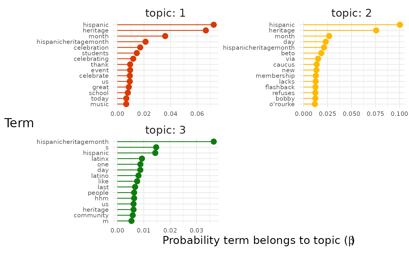
##
## [[1]]$max_only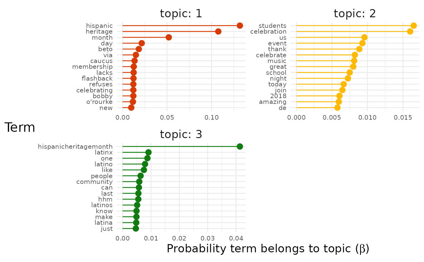
We can see that two visualisations are produced because for each
model top_terms is itself a list of two graphs.
If we just want to see one, then we can select it by name:
explore |>
  # Choose the model we're interested in
  filter(freq_cutoff == 10 & k == 3 & iter == 1000) |>
  # Choose the viz column we're interested in
  pluck("top_terms") |>
  # Choose the particular graph we're interested in
  pluck(1, "all_terms")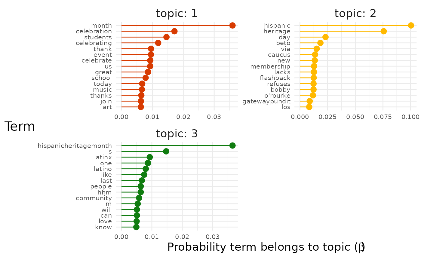
The "facetted" graph shows us the terms with the highest
probability for each topic. Sometimes this will give a clear picture by
itself of the topics in the data set.
However, we can see that the most likely terms are duplicated across topics because they represent the topic of our entire data set (in this case Hispanic Heritage Month). To get a better sense of what distinguishes the topics we can instead assign each term to the topic to which it has the maximum probability of belonging:
explore |>
  # Choose the model we're interested in
  filter(freq_cutoff == 10 & k == 3 & iter == 1000) |>
  # Choose the viz we're interested in
  pluck("top_terms", 1, "max_only")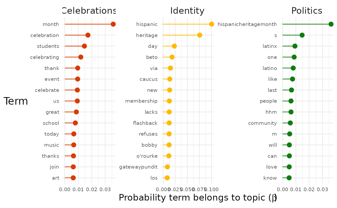
Now we get a clearer sense of the three main strands of conversation in our dataset.
- Topic 1 seems to be about literal celebrations.
- For example, terms like “event”, “music” and “food” are present.
- Topic 2 seems to be about identity and the Latinx community.
- For example, terms like “latinx”, “people”, “community” are present.
- Topic 3 seems to be about politics.
- For example, terms like “beto orourke” and “caucus” are present.
Once we’ve identified the names of the topics for the top terms plot,
we should rename them before we save the plot. We can use the
top_terms_rename function to do this:
plot <- explore |>
  filter(freq_cutoff == 10 & k == 3 & iter == 1000) |>
  pluck("top_terms", 1, "max_only")

plot +
  SegmentR::top_terms_rename(new_names = c("Celebrations", "Identity", "Politics"))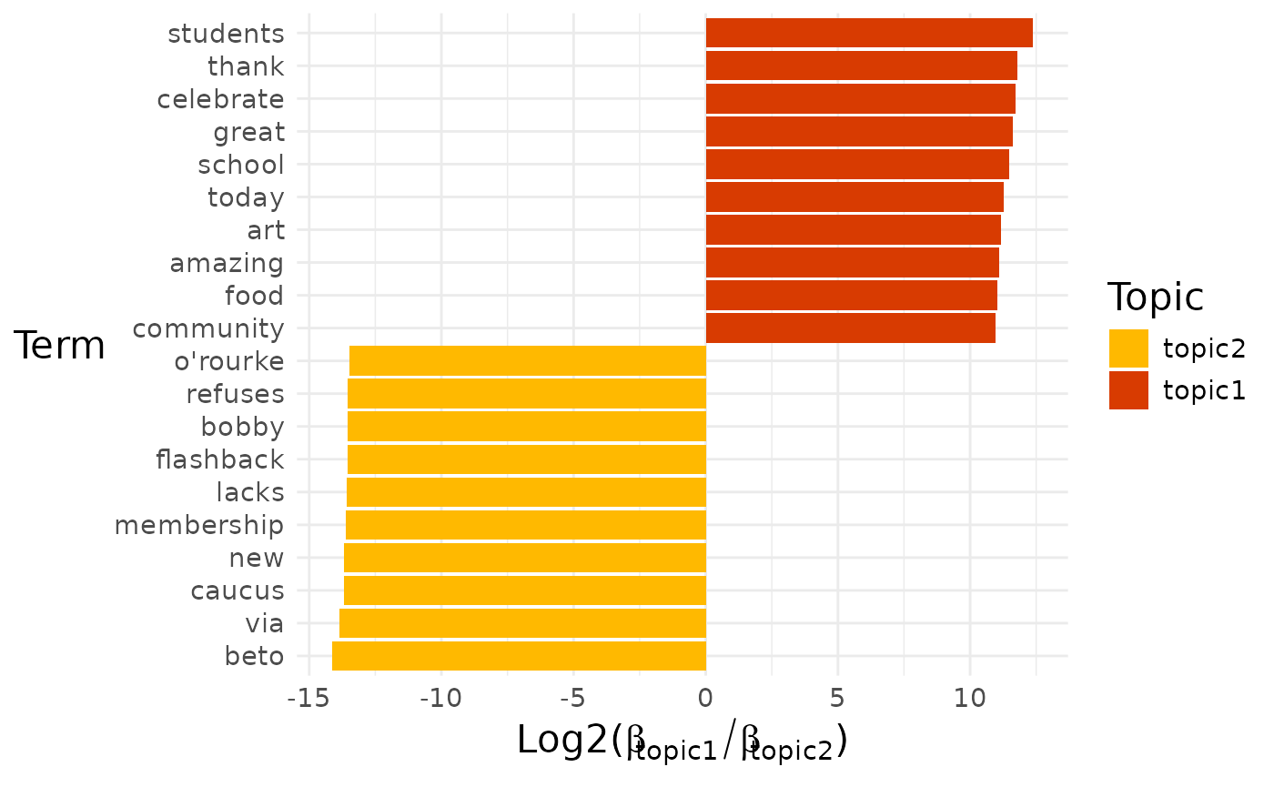
Diff terms
Sometimes we might want to know which terms distinguish two closely related topics from each other.
explore |>
  # Choose the model we're interested in
  filter(freq_cutoff == 10 & k == 3 & iter == 1000) |>
  # Choose the viz column we're interested in
  pull(diff_terms)
## [[1]]
## [[1]]$topic1_vs_topic2
##
## [[1]]$topic1_vs_topic3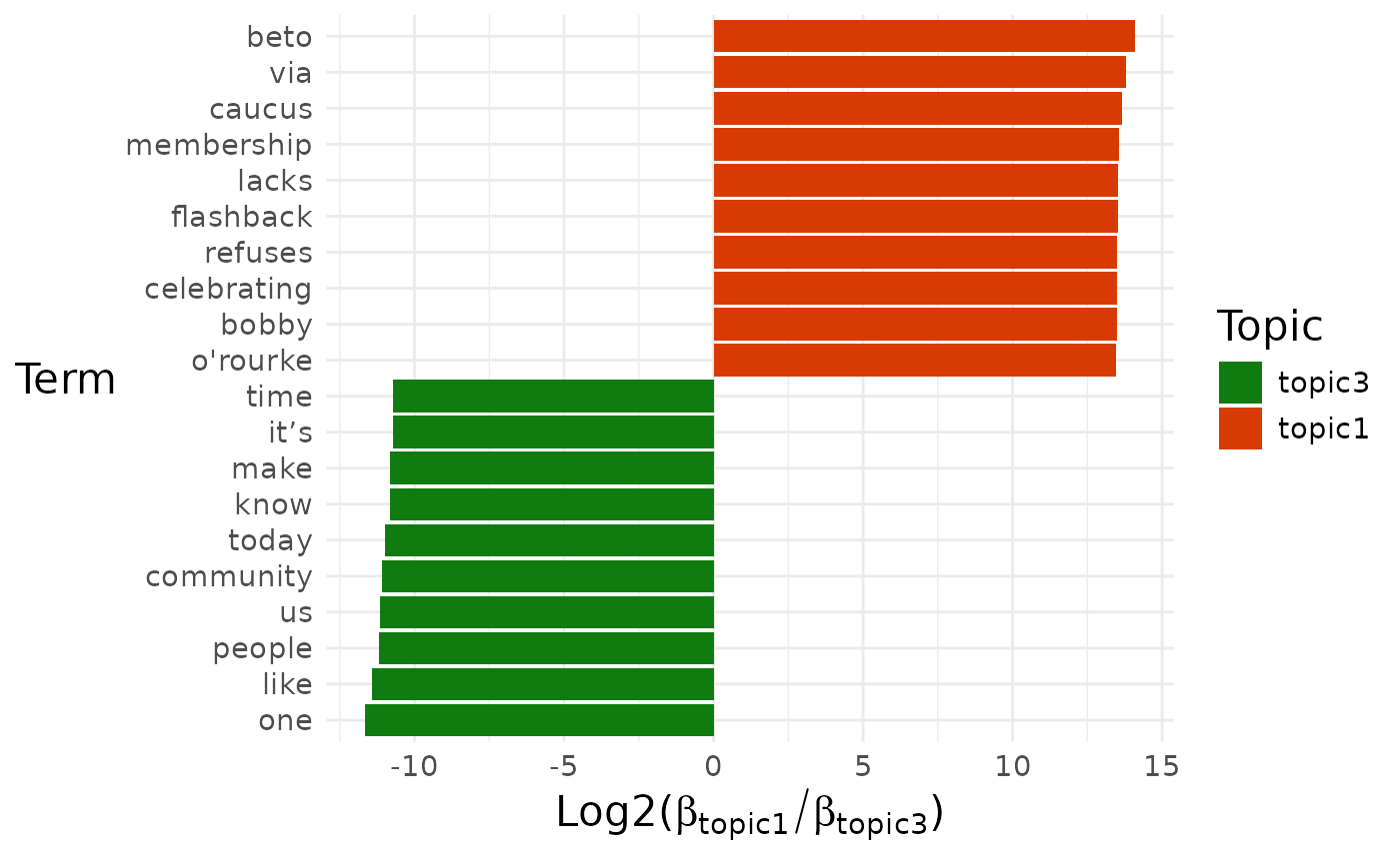
##
## [[1]]$topic2_vs_topic3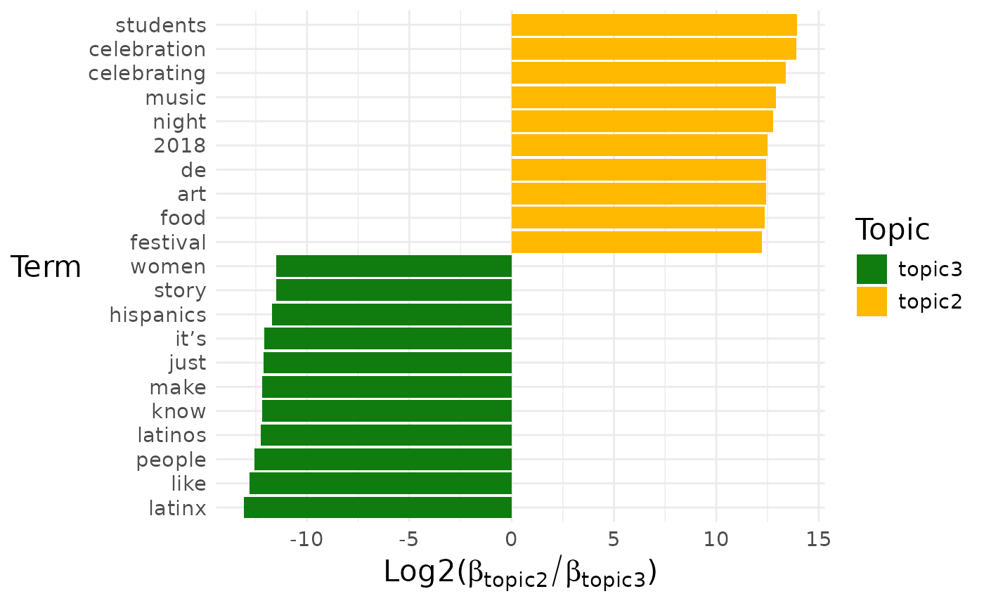
By default, a pairwise comparison for all the topics is produced.
If we want to look at a particular comparison, then we can select it by name:
explore |>
  # Choose the model we're interested in
  filter(freq_cutoff == 10 & k == 3 & iter == 1000) |>
  # Choose the viz column we're interested in
  pull(diff_terms) |>
  # Choose particular comparison
  pluck(1, "topic1_vs_topic2")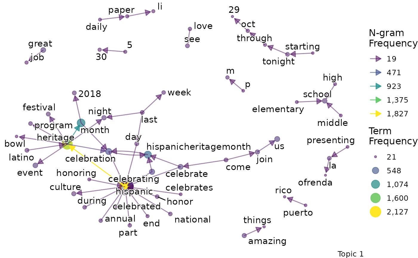
Bigrams
We might want to go beyond term frequency and look at how the terms that are representative of a topic relate to one another. To do this, we can produce bigram networks for each topic.
explore |>
  # Choose the model we're interested in
  filter(freq_cutoff == 10 & k == 3 & iter == 1000) |>
  # Choose the viz column we're interested in
  pull(bigrams)
## [[1]]
## [[1]]$topic_1_bigram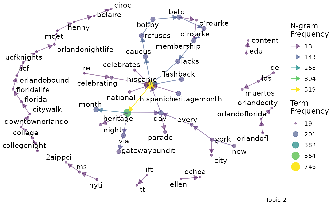
##
## [[1]]$topic_2_bigram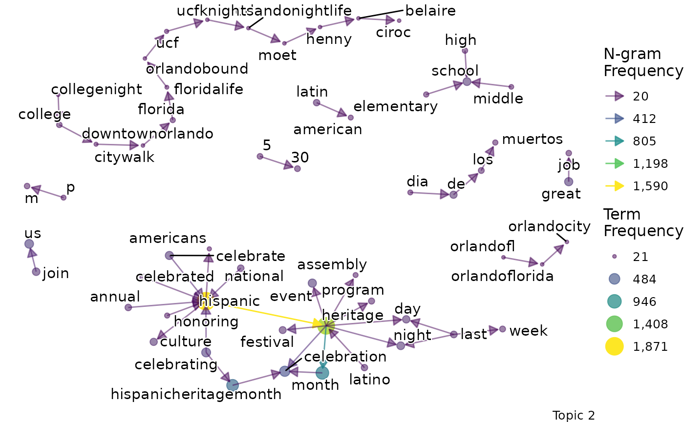
##
## [[1]]$topic_3_bigram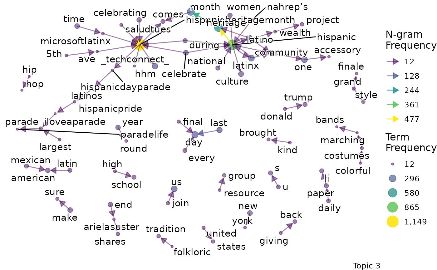
Again, a specific graph can be selected by name:
explore |>
  # Choose the model we're interested in
  filter(freq_cutoff == 10 & k == 3 & iter == 1000) |>
  # Choose the viz column we're interested in
  pull(bigrams) |>
  # Choose the particular network
  pluck(1, "topic_2_bigram")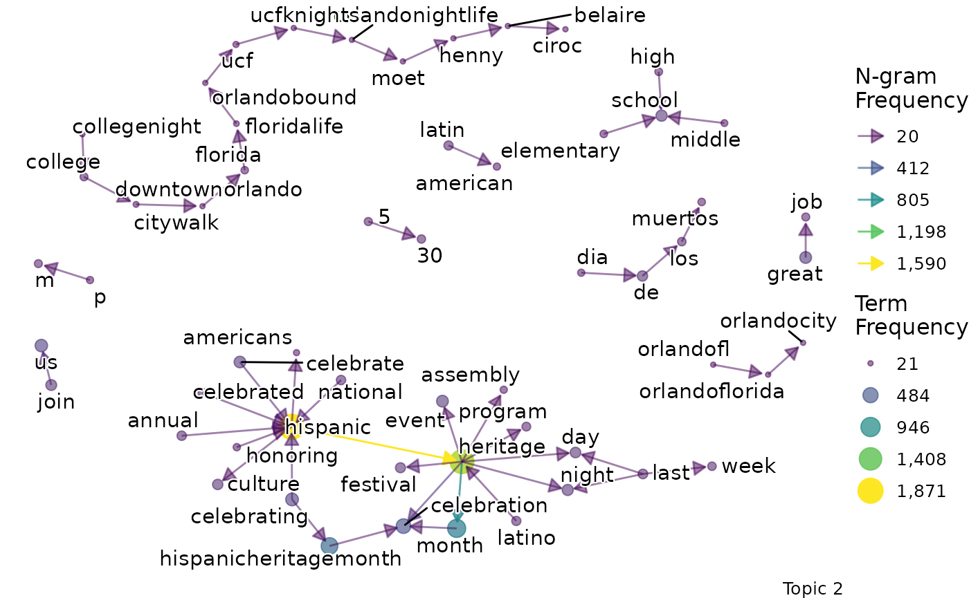
Exemplars
Once you have used the exploratory visualisations to build up an idea of what a particular topic is about, it can be useful to look at some example posts. The function returns the document from which the post came, whhich topic it is associated with, the probability it belonged to that topic, and the url to visit the original post.
Probabilities & Joining Data Frames
Here we look at how to:
- Link our topics data frame to our original data frame
- Classify our topics according to a probability threshold
- Rename our topics using a list of new topic names
You may want to find the probability that a post belongs to each topic, for every post. Knowing this information can help you determine the proportion of each topic within the full data set.
probabilities <- explore |>
  # Choose the model we're interested in
  filter(freq_cutoff == 10 & k == 3 & iter == 1000) |>
  # Choose the column we're interested in
  pluck("probabilities", 1)
The document id corresponds to the row number of the
post in the original dataframe. The probabilities tibble can be easily
binded to the original dataframe using the topics_link
function.
linked_probabilities <-
  SegmentR::topics_link(
    sprinklr_export, probabilities)
Once we have these probabilities, we can use a probability cut-off point to group the posts into topics. We can use this information to determine topic volumes, and to further examine posts within each topic.
It is up to the user to determine a suitable cut-off point by examining whether the posts display the expected information. The user also needs to take the number of topics into consideration. For example, if there are 2 topics, any probability over 0.5 (1 / 2) means that the post is more likely to belong to that topic, whereas if there are 10 topics, this base probability changes to 0.1 (1 / 10). In general, it is safer to pick a high cut-off point to increase the likelihood of posts displaying the expected information.
For example, let’s use a cut-off point of 0.7. We can determine the volume for each topic by running the following code.
topics_classified <- linked_probabilities |>
  SegmentR::topics_classify(topic_cutoff =  0.7)

topics_classified |>
  select(topic)
## # A tibble: 3,489 × 1
## topic
## <chr>
## 1 topic_2
## 2 topic_2
## 3 topic_2
## 4 topic_1
## 5 topic_3
## 6 topic_3
## 7 topic_2
## 8 topic_2
## 9 topic_3
## 10 topic_2
## # ℹ 3,479 more rowsYou can rename the topics, just input a new vector of names, starting with topic_1 and moving upwards:
topics_renamed <- topics_classified |>
  SegmentR::topics_rename(k = 3, new_names = c("celebrations",
                                     "identity",
                                     "politics"))

topics_renamed |> count(topic)
## # A tibble: 3 × 2
## topic n
## <fct> <int>
## 1 celebrations 620
## 2 identity 1579
## 3 politics 1290Coherence
Another measurement that the user might be interested in is the coherence for each topics, which tells us how associated words are within the topic. The higher the value, the more coherent the topic is. The lower the value, the more likely the words have been grouped together as a result of statistical inference.
Coherence is calculated by taking the top coherence_n
words and calculating
for each pair of words. For example, suppose the top 4 words are
.
The following are calculated:
- , , and
- and
These six values are averaged to obtain the coherence score. The
process has been automated using the textmineR package.
coherence <- explore |>
  # Choose the model we're interested in
  filter(freq_cutoff == 10 & k == 3 & iter == 1000) |>
  # Choose the column we're interested in
  pull(coherence) |>
  pluck(1)

coherence
## # A tibble: 3 × 2
## topic coherence
## <chr> <dbl>
## 1 topic_1 0.152
## 2 topic_2 0.0208
## 3 topic_3 0.0314So, in our case, the third topic is much more well-defined compared to the other two topics.
Shiny app (experimental)
the shiny_topics_explore function allows you to input an
explore object and view the top_terms, a data table of exemplars and the
bigrams for each value of k. You can use this to quickly iterate over
topics and save your notes.
The app is basic and may later be developed, depending on usage.
shiny_explore <- SegmentR::explore_LDAs(SegmentR::seg_ldas)
SegmentR::shiny_topics_explore(shiny_explore)
Tip: insert your own explore object into the
shiny_topics_explore function.