What is LDA?

The SegmentR topic modelling functions help the user to implement Latent Dirichlet Allocation (LDA). This article provides an explanation of how LDA works by using simulated data.

Overview

Say that we’ve got some documents pulled in by a broad query about science and we want to use LDA to identify underlying groups in the documents that comprise the ‘topics’ of the broader conversation.

For example, the topics might be individual fields in science like biology, chemistry, and physics.

But, crucially, we don’t know what these underlying groups are in advance. All we’ve got to work with is the content of the documents themselves.

We start by making some overarching assumptions:

Each document can contain a mixture of different topics.
- E.g. A document could be about biochemistry and therefore use words relating to biology and words relating to chemistry.
Each topic is just a collection of words that have different probabilities of appearing.
- E.g. The word “Darwin” will be more likely to occur in a document about biology than one about physics.

What we want to do is work backwards from the documents and eventually estimate probabilities relating to the two bullet points above. That is, we want to infer both:

The per-topic word distributions
- I.e. Which words characterise each topic?
- We’re trying to answer the question, “What is each topic about?”
The per-document topic distributions
- I.e. What topics characterise each document?
- We’re trying to answer the question, “What is each document about?”

Going forwards: Making documents

LDA makes some assumptions about how the documents it is trying to model were generated. It assumes that when each document was created:

The author decided how many words this document would contain.
- E.g. This document will be 5 words long.
The author chose a topic mixture for the document.
- E.g. This document will be 80% about biology, 20% about chemistry, and 0% about physics.
Each of the topics available to the author themselves contained mixtures of words.
- E.g. Biology might be comprised of 10% the word “evolution”, 5% the word “species”, and so on.
The author chose the words in the document one at a time.
- For each word they needed they:
  - Picked a topic based on the mixture of topics they had decided that document should have.
  - Picked a word based on the mixture words for that topic.

These assumptions are fairly unrealistic but turn out to be very effective.

Let’s simulate some data using the process we just described.

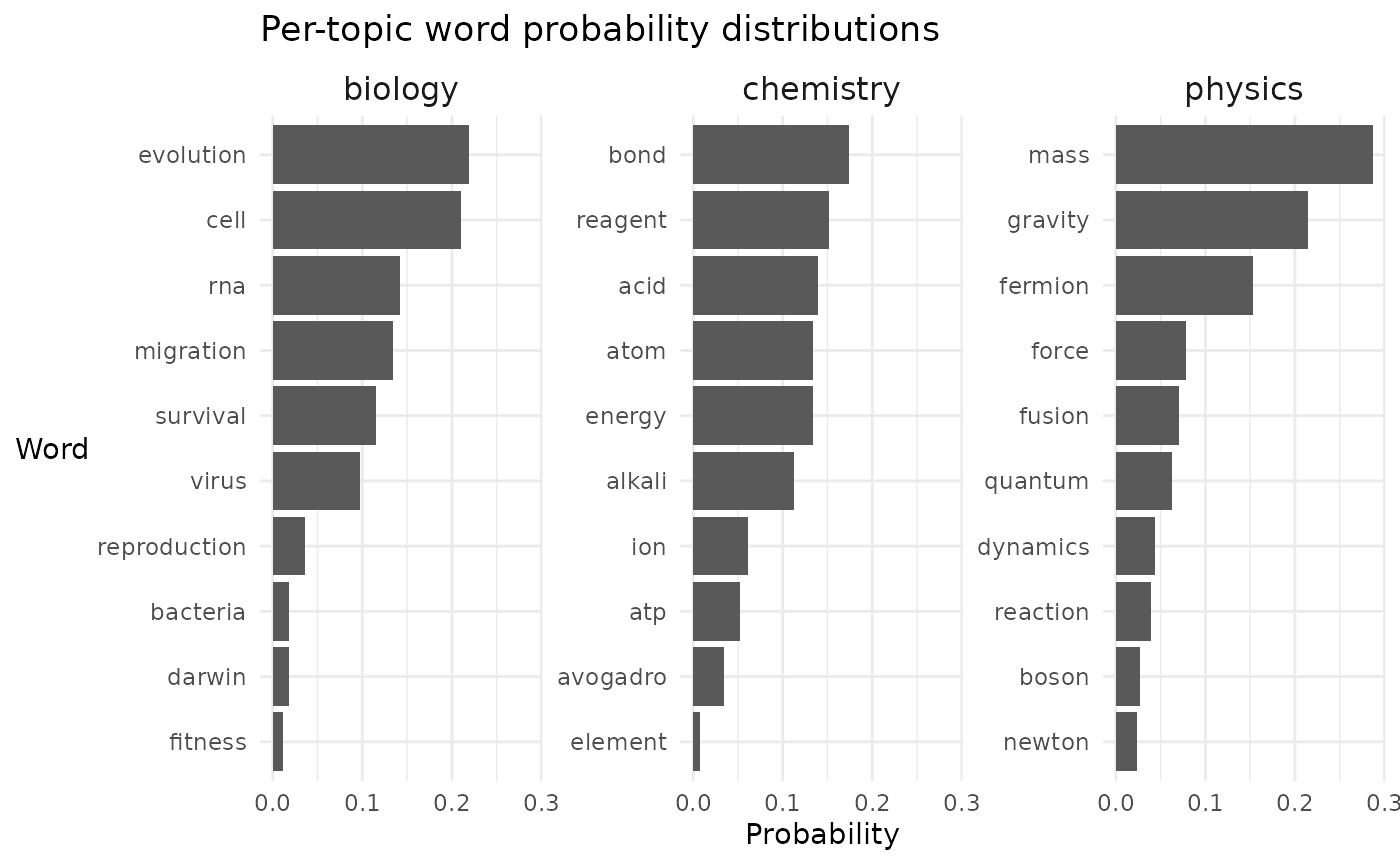
First, we need to generate the per-topic word distributions:

Second, we need to generate the per-document topic distributions:

doc_id	biology	chemistry	physics
doc_1	0.0042822	0.8607393	0.1349785
doc_2	0.0089432	0.0252095	0.9658473
doc_3	0.0069236	0.6192332	0.3738432
doc_4	0.0059822	0.9933424	0.0006754
doc_5	0.0483171	0.2960417	0.6556412
doc_6	0.1815250	0.8059074	0.0125676

Now we can generate the mock content of the documents.

doc_id	n_words	doc_content
doc_1	21	acid atp ion force bond reagent acid atom avogadro alkali mass bond acid acid gravity energy reagent energy bond acid energy
doc_2	28	fermion fusion gravity force quantum mass mass fermion gravity gravity gravity mass fusion dynamics quantum gravity dynamics gravity boson force gravity mass mass mass mass dynamics fusion gravity
doc_3	32	fermion gravity element mass atom fermion force acid bond mass energy gravity bond gravity reagent atom bond energy fermion atom fermion fermion reagent gravity alkali ion atom acid reagent bond reagent ion
doc_4	30	alkali acid acid acid alkali acid ion alkali ion reagent atom reagent energy atom acid atp atom alkali alkali reagent reagent atom bond energy bond atp reagent atp acid bond
doc_5	21	fermion atom mass quantum mass fermion force atom gravity fermion bond mass mass reaction atp fermion mass gravity reaction gravity fusion
doc_6	17	bond alkali bond bond bond reagent reagent alkali atom cell bond bond reagent bond cell energy bond

Do the words that have been selected match what you would expect given the per-document topic probabilities in the previous table?

Going backwards: Finding topics

Now that we’ve simulated some idealised documents, we can work through the process we’d actually complete for a client project. That is, we can work backward from the document content to find topics.

To understand how LDA works, pretend that all but a single word in a single document was correctly assigned to its respective topic. How could we decide what topic we should assign to this final word?

One way to guess is to consider two questions:

How often does the word appear in each topic elsewhere?
- If the word often occurs in discussions of one topic, then this instance of the word probably belongs to that topic as well.
But a word can be common in more than one topic.
- E.g. We don’t want to assign “lead” to a topic about leadership if this document is mostly about heavy metal contamination.
So we also need to consider, How common is each topic in the rest of this document?
- E.g. Are the other words in this document mostly leadership terms or names of other metals?

This is what the LDA algorithm essentially does. For every word, it creates, for each possible topic, a measure that takes into account the answers to the above two questions and then assigns the word to the topic with the highest score on this measure.

If, instead of having the problem virtually solved, we had only a random guess about which word belonged to which topic, then we could still use the same strategy.

We go through the collection, word by word, and reassign each word to a topic, guided by the two questions above.
As we do:
- Words become more common in topics where they are already common.
- Topics become more common in documents where they are already common.
Our model becomes gradually more internally consistent.

Remember, all we have to work with is the document content:

doc_id	doc_content	permalink
doc_1	acid atp ion force bond reagent acid atom avogadro alkali mass bond acid acid gravity energy reagent energy bond acid energy
doc_2	fermion fusion gravity force quantum mass mass fermion gravity gravity gravity mass fusion dynamics quantum gravity dynamics gravity boson force gravity mass mass mass mass dynamics fusion gravity
doc_3	fermion gravity element mass atom fermion force acid bond mass energy gravity bond gravity reagent atom bond energy fermion atom fermion fermion reagent gravity alkali ion atom acid reagent bond reagent ion
doc_4	alkali acid acid acid alkali acid ion alkali ion reagent atom reagent energy atom acid atp atom alkali alkali reagent reagent atom bond energy bond atp reagent atp acid bond
doc_5	fermion atom mass quantum mass fermion force atom gravity fermion bond mass mass reaction atp fermion mass gravity reaction gravity fusion
doc_6	bond alkali bond bond bond reagent reagent alkali atom cell bond bond reagent bond cell energy bond

And we want to infer both:

The per-topic word distributions
- I.e. Which words characterise each topic?
- We’re trying to answer the question, “What is each topic about?”
The per-document topic distributions
- I.e. What topics characterise each document?
- We’re trying to answer the question, “What is each document about?”

The most common use case at SHARE only involves answering the question, “What is each topic about?” so we’ll just focus on finding the per-topic word distributions in our simulated documents.

Using `SegmentR` functions

First let’s see how well the SegmentR functions do with this simulated data.

Convert into dtm:

dtm <- make_DTMs(df = real_documents,
                 text_var = doc_content,
                 url_var = permalink,
                 min_freq = 1)

Run the LDA algorithm:

set.seed(1)
lda <- fit_LDAs(dtms = dtm,
                k_opts = 3, # In reality, we would have to test different values for k
                iter_opts = 10000)

Add just the top terms graphs for this model so that we can explore the per-topic word probabilities:

explore <- explore_LDAs(ldas = lda,
                        top_terms = TRUE,
                        top_n = 10,
                        diff_terms = FALSE,
                        bigrams = FALSE,
                        exemplars = FALSE)

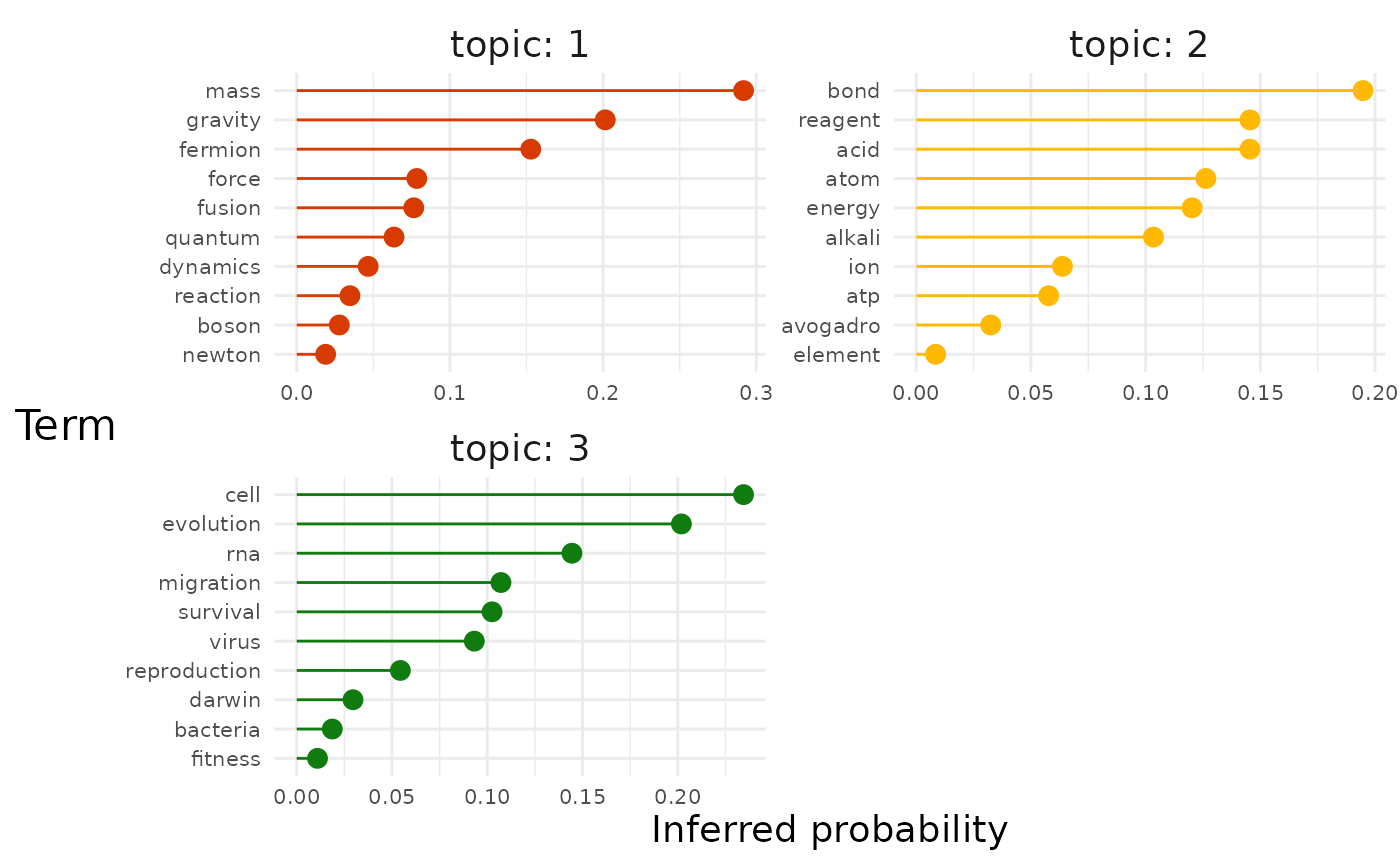
Let’s have a look at top terms for each topic first:

How do the inferred per-topic word probabilities measure up to what we know they actually are?

Not bad at all. The model doesn’t get the order right for each topic but generally captures which terms are high probability and low probability (e.g. For biology, “cell” and “evolution” vs. “darwin” and “fitness”).

Work through the algorithm manually

Reassuringly the LDA functions in SegmentR did a good job on our neat simulated data.

But what literal process are the functions working through? Let’s play through a simplified version manually that will clarify the logic.

We saw that we used SegmentR::make_DTMs() to create a document-term matrix. To make things clearer let’s build a tibble containing the same information where each document is broken down into individual words:

doc_id	permalink	word
doc_1		acid
doc_1		atp
doc_1		ion
doc_1		force
doc_1		bond
doc_1		reagent

Randomly assign each word a topic:

word_id	doc_id	word	topic
1	doc_1	acid	1
2	doc_1	atp	3
3	doc_1	ion	1
4	doc_1	force	2
5	doc_1	bond	1
6	doc_1	reagent	3

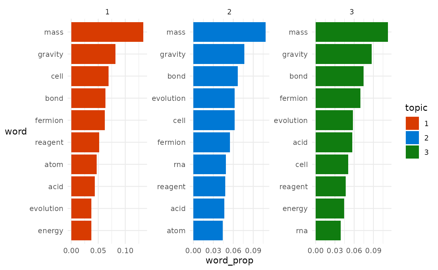
Our starting point with randomly assigned topics looks suitably nonsensical:

Let’s start trying to improve our assignments.

Select a random word in a random document.

word_id	doc_id	permalink	word	topic
1017	doc_40		fusion	3

We’ve got the word fusion from document 40 which has randomly been assigned topic 3.

Now, for each topic \(t\) we need to calculate two proportions that correspond to the two guiding questions we discussed earlier:

How often does the word appear in each topic elsewhere?
- Proportion of assignments to topic \(t\) over all the documents that come from the word “fusion”.
  - \(Pr(\text{Word}\; w|\text{Topic}\; t)\)

# Find proportion of assignments to each topic across all documents that come from "fusion"

# - Total assignments to each topic
assignments_total <- random_topics %>%
  count(topic, name = "n_total")

# - Assignments to each topic due to the word "fusion"
assignments_from_word <- random_topics %>%
  filter(word == selected$word) %>%
  count(topic, name = "n_from_word")

# - Proportion of total assignments due to "fusion"
assignments_prop <- left_join(assignments_total, assignments_from_word) %>%
  mutate(prop_from_word = n_from_word/n_total) %>%
  select(-n_total, -n_from_word)

How common is each topic in the rest of this document?
- We find the proportion of words in document 41 that are currently assigned to topic \(t\).
  - \(Pr(\text{Topic}\; t|\text{Document}\; d)\)

# Find proportion of words in document that are assigned to each topic
per_doc_topic <- random_topics %>%
  filter(doc_id == selected$doc_id) %>%
  count(topic) %>%
  mutate(prop_from_topic = n/sum(n)) %>%
  select(-n)

Next, we combine our answers to these questions.

Multiply the proportions to create a measure of how much we think we should assign this instance of “fusion” to each topic.
- \(Pr(\text{Topic}\; t|\text{Document}\; d) \times Pr(\text{Word}\; w|\text{Topic}\; t)\)

# Multiply these proportions for each topic
final_probs <- left_join(per_doc_topic, assignments_prop) %>%
  mutate(outcome = prop_from_topic * prop_from_word)

topic	prop_from_topic	prop_from_word	outcome
1	0.3939394	0.0328253	0.0129312
2	0.3030303	0.0322581	0.0097752
3	0.3030303	0.0278129	0.0084282

Finally, we assign the word to the topic with the highest score.

# Assign the word the topic with the highest value
new_topic <- final_probs %>%
  filter(outcome == max(outcome)) %>%
  pull(topic)

slightly_less_random_topics <- random_topics %>%
  mutate(topic = replace(topic, word_id == selected$word_id, new_topic))

Now imagine we run through that same process 30,000 times slowly improving our topic assignments.

We can visualise the top 10 terms assigned to each topic to see how this simplified version of the algorithm with 30,000 runs did:

How do they compare to the actual per-topic word probabilities we simulated?

Physics is spot on, Chemistry is pretty good, and Biology is mediocre.

On the whole this outcome is still fairly impressive considering we’re just following a simplified version of algorithm and started with completely random guesses.

Overview

Going forwards: Making documents

Going backwards: Finding topics

Using SegmentR functions

Work through the algorithm manually

Further reading

Using `SegmentR` functions