This is a copy of a SHARE white paper outlining a framework we refer to as MeasureR.
Introduction
The problem
Answer the following question for me:
How tall are you?
Whether you’re a gymnast or a basketball player, you have a variety of units to choose from for your answer. You could answer in metres, in feet & inches, or, if you’ve got four legs and a long face, in hands. The wide variety of units available to you is a consequence of the fact that height is a well-defined and measurable variable.
Now, try this one:
How relevant is your product to your customers?
Do any common units come to mind?
This example illustrates the idea that key business outcomes aren’t always well-defined and easily measurable variables. Sometimes they’re big vague concepts. That’s a problem if you want to model them.
One approach to solving this problem might be to break down a question about a vague concept into smaller questions involving well-defined variables. For example, the overarching question, “Did our latest campaign improve our product’s relevance?”, might be split into questions like, “Did our latest campaign have a higher click-through rate than our historical average?”.
However, you end up with answers to a variety of small questions about ‘relevance’ and have to decide how to patch the findings together yourself. Even worse, one analyst might combine them slightly differently from another.
Our solution
Although we can’t say what units we would measure our vague business outcome in, we do have a sense of what we mean by concepts like ‘relevance’. We also have ideas about what variables might increase or decrease it. It turns out this is all you need to improve your decision-making.
MeasureR: A straightforward approach to modelling business outcomes using improper models.
- Measure your intuition to improve the accuracy and reliability of your decision-making.
To show you what this looks like in practice, our CEO Ian Cassidy used our MeasureR framework to develop a custom metric to measure a vague, but important, personal outcome: his household’s happiness.
Background
Just like anyone else trying to develop a model, Ian had three broad frameworks to choose from:
- Intuition
- Proper Modelling
- Improper Modelling
The accuracy of each of these approaches is determined by the combination of human and algorithmic decision-making involved. Generally, humans are good at selecting the most relevant variables to consider, but bad at combining them to make a decision, whereas algorithms are the opposite. With these relative strengths in mind, let’s consider each modelling framework in turn.
Intuition
With an intuitive modelling approach, an expert’s gut instinct is used to make predictions and decisions about the outcome of interest.
As a member of his household, Ian is probably a qualified expert in its ‘happiness’. He could simply give every day an intuitive rating, and track how these ratings change over time.
However, such intuitive models are often the least accurate approach to take. Although Ian would be playing to his human strength in choosing the relevant variables, he would also be exposing his human weakness by (probably) combining the variables non-optimally and inconsistently. Further, the whole ‘modelling process’ is an unconscious thought process meaning its rationale can’t be inspected.
So, going ‘full human’ when trying to model a vague outcome probably isn’t the best approach. Let’s look at the opposite end of the spectrum next.
Proper models
With a proper modelling approach, supervised learning techniques are used to train a model which can make predictions about the outcome of interest.
As CEO of a company with in-house data scientists, Ian has easy access to these fancy machine learning techniques and could use them to create a proper model of his household’s ‘happiness’.
Proper models are often the most accurate type of model because they play to both humans’ and algorithms’ strengths with the former choosing the relevant variables and the latter combining them optimally and consistently. Here, ‘optimally’ refers to the fact that proper models use a formal optimisation process where some measure of the model’s utility is maximised or minimised. For example, in a simple linear regression the sum of the squared residuals is minimised.
However, there are two stumbling blocks for Ian’s potential proper model of household happiness. The first is that the most accurate methods are often flexible machine learning techniques which can be difficult to interpret and implement. There’s not much benefit to Ian in modelling household ‘happiness’ perfectly if his model’s reasoning process is so convoluted that he can’t use it to try to make tactical improvements. The second, more fundamental, problem is that proper models require a well-defined, measurable outcome variable. ‘Happiness’ doesn’t really fit the bill here. What units do you measure ‘happiness’ in? Perhaps Ian could try using a survey as a proxy or, depending on his financial commitment to this pet project, daily fMRI imaging. In either of these examples, the daily measurement itself would probably have a negative impact on ‘happiness’ (however you measure it), and they’d still only be proxies so there’d be little point.
It seems that relying on an algorithmic approach when modelling a vague outcome won’t work either. So far the two approaches we’ve covered have been too hot and too cold, too hard and too soft. Now, let’s discuss one that’s just right.
Improper models
Improper models provide a simple decision rule to make predictions about the business outcome that we’re interested in. They combine variables without using optimisation to decide how to weight the importance of each.
As we alluded to in the previous section, an improper modelling approach is a Goldilocks zone. It’s more accurate than intuition and more tractable than proper modelling. Their accuracy tends to be better than intuition alone because the variables are being combined using an algorithm that, despite being non-optimal, is consistent and inspectable. This means there will be no noise in Ian’s decision-making and he can tweak his approach based on results over time. Their tractability comes from the fact that they do not require optimisation and can be used with a vague outcome variable like ‘happiness’.
Ian decided an improper model was a sensible approach for measuring, tracking, and eventually improving household ‘happiness’. So, how did he make one?
Implementation
Ian took three steps to define his improper model:
- First, he had to choose which variables to include.
- Second, he had to format the variables so that they were directly comparable and had the right kind of relationship with ‘happiness’.
- Third, he had to give each variable a weight to denote its importance.
Pick the variables
The foundation of the improper modelling process is pre-existing client expertise. Once we’ve settled on a business outcome, then we’d collaboratively decide:
- The most important variables to include as predictors of the outcome
- Whether each variable has a positive or negative relationship with the outcome.
Ian settled on the following 3 variables:
children_argue
The number of times his children argued with each other in a week.
Ian decided this variable had a negative relationship with household happiness.
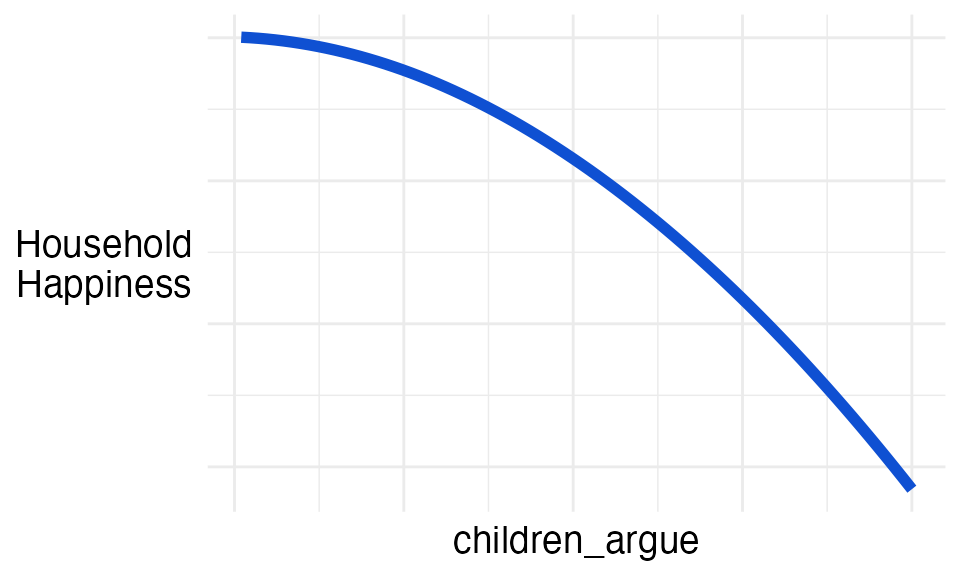
That is, the more his children argue, the less happy the house is.
spousal_affection
We’ll leave this definition to your imagination.
Ian decided this variable had a positive relationship with household happiness.
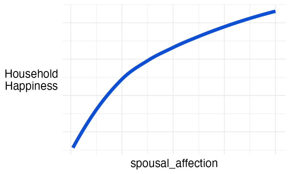
After all, more is always better.
meals_together
The number of meals in a week that are eaten together as a family.
Ian decided this variable had a ‘one-hump’ relationship with household happiness.
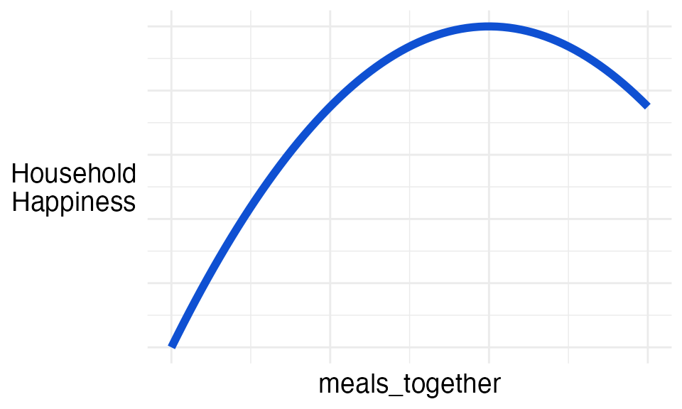
More dinners together increases with household happiness up to a point. But, after this maximum, more dinners together accompanies a decrease in household happiness. For example, too many dinners together could signal that family members have not seen their friends in a while.
Format them
So, Ian had the 3 variables he believed contributed to household
happiness: children_argue, spousal_affection,
and meals_together. He had also decided what the general
relationship between each variable and happiness was.
However, he still had two problems.
- First, Ian knew from his favourite psychometrics textbook that for
an improper linear model to work each variable needs to have a
conditionally monotonic relationship with the outcome.
- This means that as the value of the variable increases the expected value of the outcome increases or decreases continuously (i.e. the relationship is a smooth line that either always goes up or always goes down).
- So, he needed to format the
meals_togethervariable so that instead of having ‘one-hump’ where the relationship switches from positive to negative it continuously increased or decreased.
- Second, the variables weren’t on the same scale.
- That is, the same number didn’t represent the same magnitude.
- For example, a value of 7 for
children_argueis a pretty run-of-the-mill week, but a value of 7 forspousal_affectionis good going by anyone’s standards. - So, he needed to standardise each variable so that they represent differences from their mean (i.e. how above or below average this week’s value is).
- This step would be even more important if the variables were measured in different units like height and weight as it would ensure that the values were now ‘unit-free’.
Monotonicity
We saw earlier that Ian suspected meals_together had a
‘one-hump’ relationship with household happiness.
To give you a little more detail, Ian thought that 10 meals together per week coincided with maximum happiness.
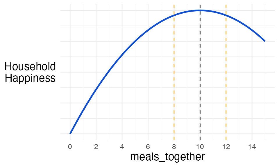
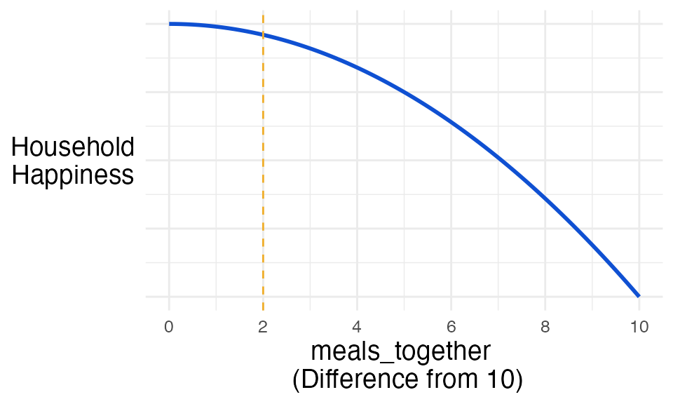
So, he needed to transform the variable so that its relationship with
happiness either continuously increased or decreased. For example, he
needed meals_together to have the same effect in his model
when it had a value of 8 as when it had a value of 12. These two values
(shown by the dashed orange vertical lines) should have the same effect
because both are the same distance away from the peak value of 10.
To do this, we find the absolute difference between each value of the variable and the value at the peak of its relationship with the outcome.
\[x_\text{diff_from_peak} = |x - x_{\text{peak}}|\]
In Ian’s case:
\[\text{meals_together}_\text{diff_from_10} = |x - 10|\]
The values now measure closeness to the peak of the relationship with the outcome. So if we plug in our examples of 8 and 12 from before we see we get the equivalence we were looking for:
\[\begin{aligned} \text{meals_together}_\text{diff_from_10} &= |8 - 10|\\ &= |-2| \\ &= 2 \end{aligned}\]
\[\begin{aligned} \text{meals_together}_\text{diff_from_10} &= |12 - 10|\\ &= |2| \\ &= 2 \end{aligned}\]
Once we’ve performed this transformation, we have the conditionally monotonic relationship we’re looking for:
Standardisation
To convert our variables to the same scale, we standardise them. There are a variety of methods available. The most common method is to subtract the variable’s mean from each observation and then divide by the variable’s standard deviation.
\[x_{\text{norm}} = \frac{x - \mu}{\sigma}\]
For example, using 10 weeks of Ian’s data for the
children_argue variable.
## [1] 2 2 4 4 5 6 6 6 7 1He standardised the values using the formula above. Now, the values measure (in standard deviations) how far away each week’s argument count is from the mean.
## [1] -1.12 -1.12 -0.15 -0.15 0.34 0.83 0.83 0.83 1.31 -1.60He did this for all three variables so that they could be combined and compared.
Weight them
Ian was almost there. He had chosen his variables, he had decided their relationships with the outcome, he had transformed them so they were monotonic, and he had standardised them. All that remained was to choose how to weight each variable’s importance (remember, this is necessary because we’re not using optimisation to generate the weights automatically as we would with a proper model).
He had three options to choose from:
Equal Weights
He could give all three variables the same weight if he believed they were equally important. This is as simple as it sounds. He would just add the transformed, standardised variables together giving a final model of household happiness as:
\[\text{happiness} = \frac{1}{3}\text{spousal_affection}_\text{norm} - \frac{1}{3}\text{meals_together}_\text{diff_from_10_norm} - \frac{1}{3}\text{children_argue}_\text{norm}\]
Intuitive Weights
Alternatively, Ian could use subject-matter expertise to give weights
which assign the relative importance of each variable. For example, if
he believed that children_argue was twice as important as
the other two variables, then he would assign it a weight that was twice
as large.
\[\text{happiness} = \frac{1}{4}\text{spousal_affection}_\text{norm} - \frac{1}{4}\text{meals_together}_\text{diff_from_10_norm} - \frac{1}{2}\text{children_argue}_\text{norm}\]
Bootstrapped Weights
Finally, if Ian had a pre-existing metric that he trusted like a survey, then he could assign weights to replicate this metric. Using this method would allow him to explain his trusted measure in terms of the variables he had chosen and mimic its predictions in the future.
\[\text{happiness} = \frac{1}{?}\text{spousal_affection}_\text{norm} - \frac{1}{?}\text{meals_together}_\text{diff_from_10_norm} - \frac{1}{?}\text{children_argue}_\text{norm}\]
Use your metric
Once Ian had defined his custom metric for happiness, all that remained was to use it.
So, for the past year Ian diligently collected the data required and measured his household’s happiness over time (Yes, as his wife smoked a cigarette, he typed “+1” in an excel spreadsheet).
Let’s visualise the results:
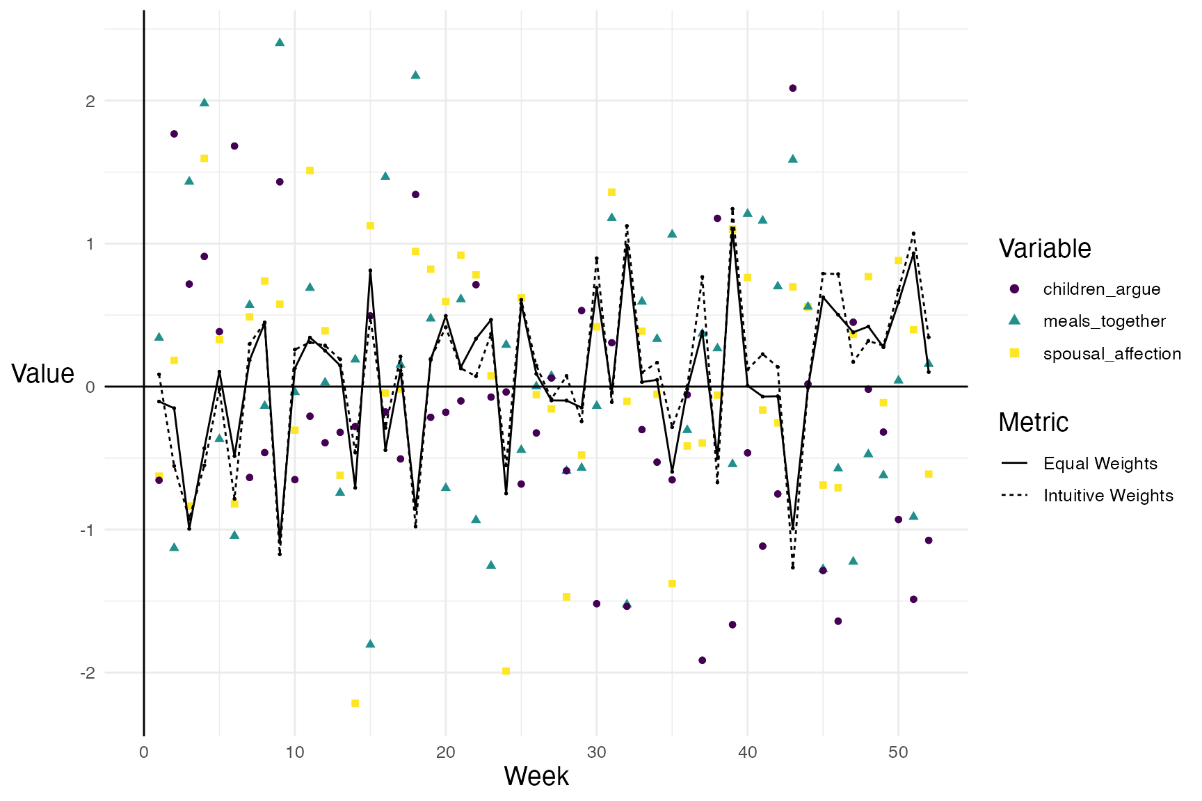
The graph illustrates how the two different weighting options combine the same data in a slightly different way to give a different outcome. Both lines have been included here to emphasise the role of the weighting choice but, in reality, there’d only be one.
What is hopefully clear is that Ian has been able to quantify, measure, and track the vague variable ‘happiness’. He has successfully completed a key goal of all data analysis by making an important variable measurable rather than falsely elevating unimportant variables that are easy to measure. That is, by using the MeasureR framework he’s made the important measurable, not the measurable important.
We can even use the data to create interactive graphs for a live dashboard so that Ian can hover over any of the points or lines to understand more intuitively how the values change over time.